Contents
Download
Description
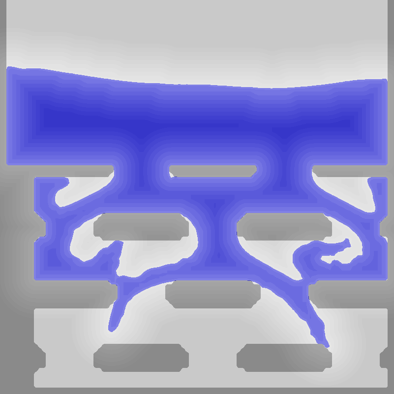
“FEM Fluid” is an experimental fluid simulation using the finite element method for pressure projection. This project is implemented in Matlab with an own FEM solver creating videos of 2D scenarios. This student project was part of my studies at TU Wien and supervised by Christian Hafner.
Fluid Simulation
Fluids can be described with the Navier-Stokes equations:
\(\frac{\partial \mathbf{u}}{\partial t} + \mathbf{u} \cdot \nabla \mathbf{u} + \frac{1}{\rho} \nabla p = \mathbf{g} + \nu\nabla \cdot \nabla\vec{u}\)
\(\nabla \cdot \mathbf{u} = 0\)
Where:
- \(\vec{u}\): velocity in m/s, as vectors in a velocity field
- \(t\): time in s
- \(\vec{g}\): external forces in kg*m/s2, for example gravity
- \(\vec{\rho}\): density in kg/m3
- \(p\): pressure (force per area) in kg/(m*s2)
- \(\nu\): dynamic viscosity (resistance against deformation) in kg/(s*m)
The upper equation describes how the fluid reacts to forces, which is basically like the Newtons equation F=m*a. The lower equation keeps the fluid divergence-free, which means that no fluid is created or destroyed.
There are two fundamental views for fluid simulations: Lagrangian and Eulerian. The Lagrangian approach is to simulate the fluid with particles. Simply put, the information about the fluid moves with these particles. PCISPH by Barbara Solenthaler is a very good algorithm using this approach. In the Eulerian approach, the information about the fluid is given at fixed positions, usually at grid nodes. Our application uses the Eulerian approach.
Advection
In short, advection is the movement of the fluid within the domain (the simulation area). The two implemented advection algorithms are Semi-Lagrangian and MacCormack’s method. Semi-Lagrangian is simply a linear movement with constant velocity. MacCormack’s is much more accurate through an error estimation and correction step.
Pressure Projection
Pressure projection is the process of making the fluid divergence-free. We want to simulate water under normal conditions. Therefore, we drop the compressibility and viscosity terms, and simplify the Navier-Stokes equations to:
We solve these equations by using the finite element method (see next section). The result is the current pressure field. We calculate the pressure gradient with finite differences (central, forward, and backward differences). Then, we subtract the pressure gradient from the current velocity field and – if the solution is accurate – receive a new, divergence-free velocity field.
Finite Element Method
The finite element method (FEM) is a numerical technique to solve certain partial differential equations. We use it to solve the incompressible Navier-Stokes equations. Simply put, we subdivide our large simulation area into many small parts, called cells. Cells are made of nodes. In our application, these nodes are the grid nodes. Finding a partial solution for each cell and then combining them is much easier than finding the entire solution at once.
In the context of fluid simulation, we create a ‘local’ matrix for each cell, which models the pressure influence of each node. Since air has a much lower density than water, we simply ignore all completely air-filled cells. In mixed cells containing fluid and air, we set the influence of air nodes to zero. Completely solid-filled cells can also be ignored. Mixed cells containing solid and fluid nodes are treated like completely fluid-filled ones. The only difference is that the velocity of solid nodes is set the object’s local velocity, which is zero in our application. All ‘local’ matrices are combined to a ‘global’ matrix. This ‘global’ matrix is sparse because only few elements around the diagonal are non-zero. In our application, Matlab solves this large matrix giving us the pressure field. If you want your own solver, the Jacobi iteration is probably the easiest algorithm. When using other algorithms, make sure the matrix is numerically stable, e.g. through pivoting.
Boundary Conditions
Boundary conditions describe how the fluid interacts with other fluids or solid objects. Other fluids can be more viscous (honey) or less viscous (alcohol, air). The friction at fluid-solid interfaces determines if the fluid can slip along the solid. In other words, the fluid at an object can have a different velocity than the object. When the friction is zero, the boundary condition is ‘free-slip’. When the fluid should have the same velocity as the object, the boundary condition is ‘no-slip’. It is also possible to have a mixture of both. In our case, we use ‘free-slip’, which is already included in the incompressible Navier-Stokes equations.
How to start
Run the main.m in Matlab. Don’t forget to switch to the current directory. In the main, you can change settings like:
- Grid resolution
- Physical size of grid cells
- Number of simulation steps
- Passed time between steps
- Advection algorithm: Semi-Lagrange or MacCormack’s
- Advection interpolation: nearest neighbor, linear, cubic, or spline
- Dissipation
- Scenario
- Several visualization settings
Known Issues
This FEM Fluid simulation suffers from instability and fluid loss. The instability occurs when the fluid almost comes to rest and causes strange movement. The reasons are probably either numerical issues or bugs. The fluid loss is caused by inaccuracies of the FEM pressure solver and fundamental issues with high velocities in the advection. Both effects are described more precisely in the Documentation and Report.
Update 30.11.2016: The instability mostly results from using ‘cubic’ or ‘spline’ interpolation for the advection. ‘linear’ causes almost no instability but slightly higher volume losses in the advection part.